Usage Examples
In this page some examples showing some features of the tool. Examples are found in the folder SensorPlacement/examples.
Increasing problem difficulty
We consider increasing the difficulty of the problem with more stringent frequency domain requirements. We run the sensor placement algorithm increasing the size of the annulus, increasing the value  . We let
 Kmin fixed to  . We design arrays for increasing
 Kmax in 
We consider circular uniform possible positions with N: 205.
In all cases we set TimeLimit: 600 and use 32 processors.
Kratio=2
Here we use  . This is an easy problem and a really good array is found.
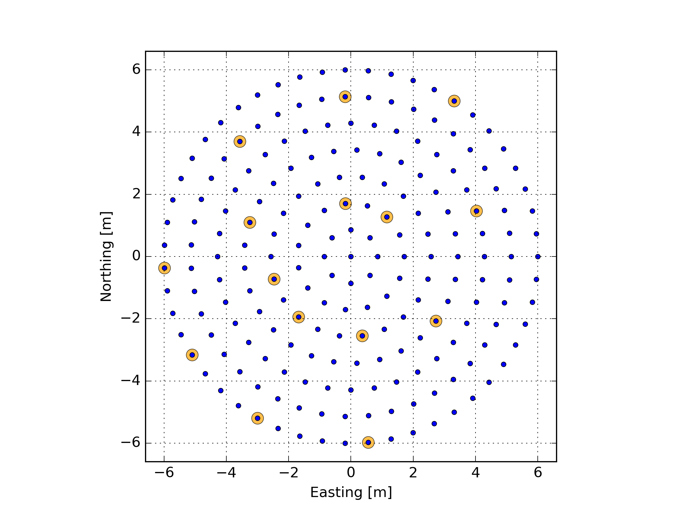
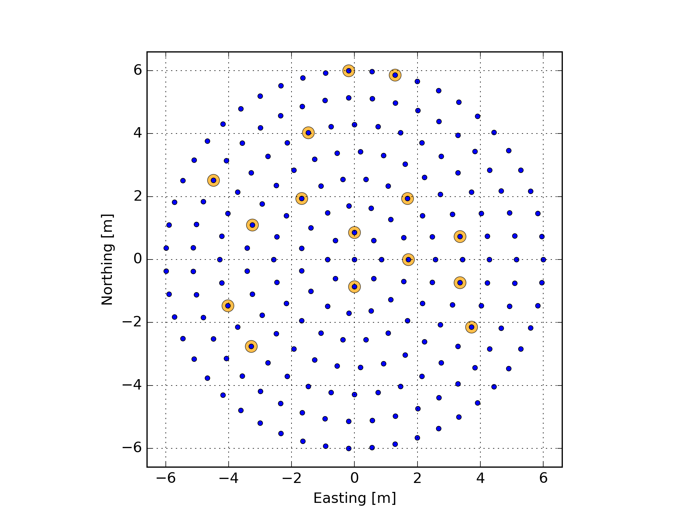
Possible sensor positions and optimized array.¶ |
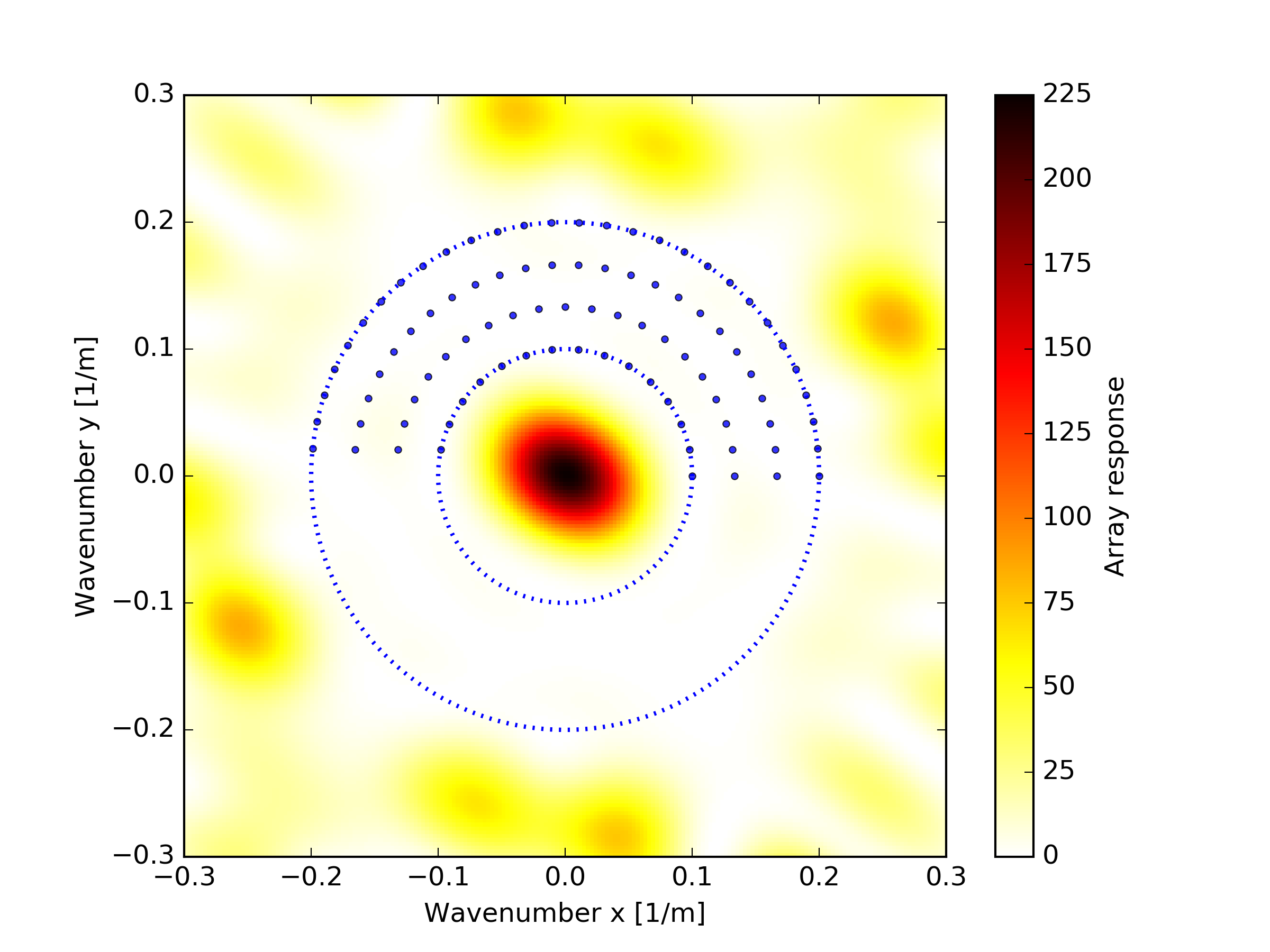
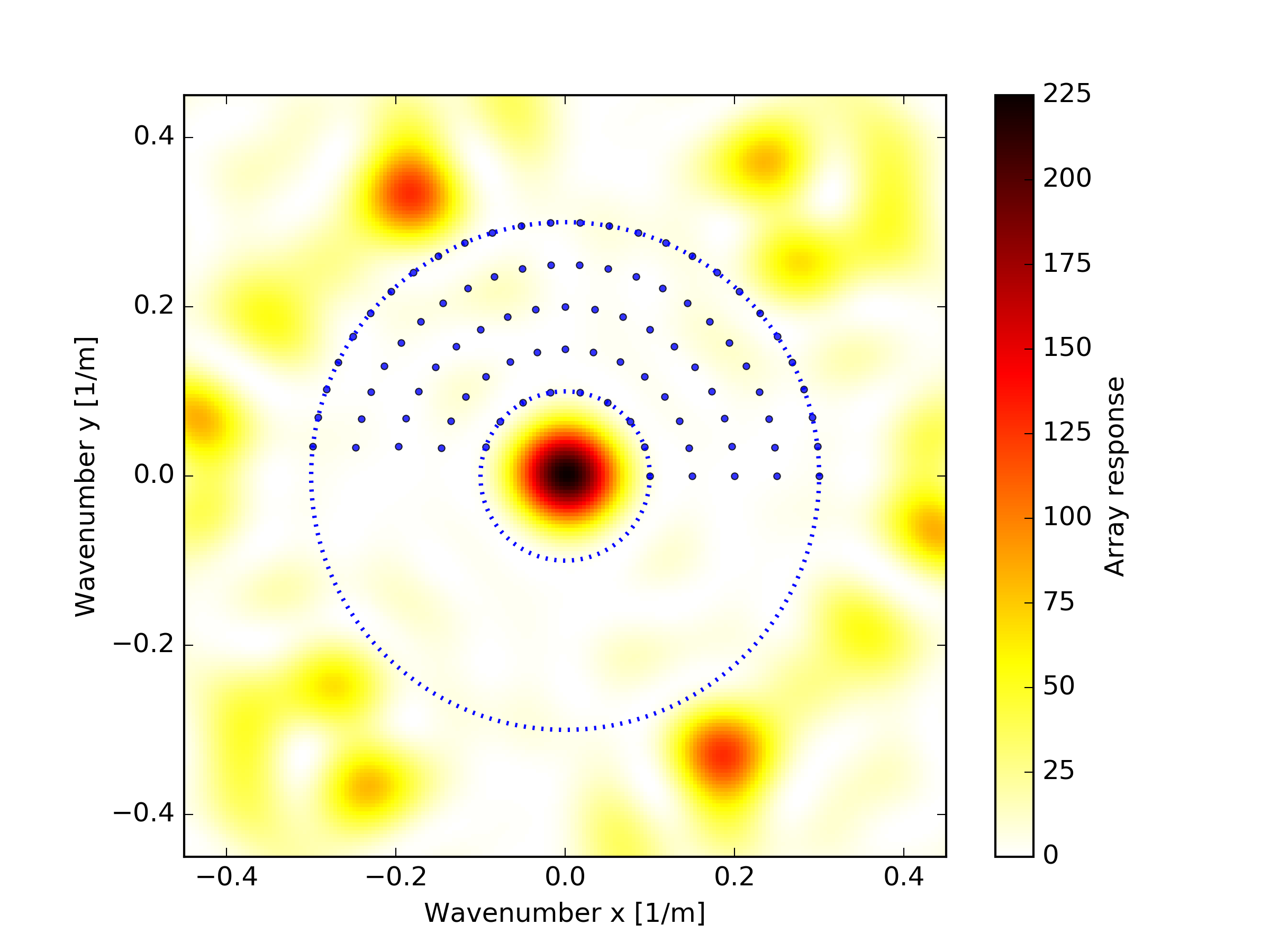
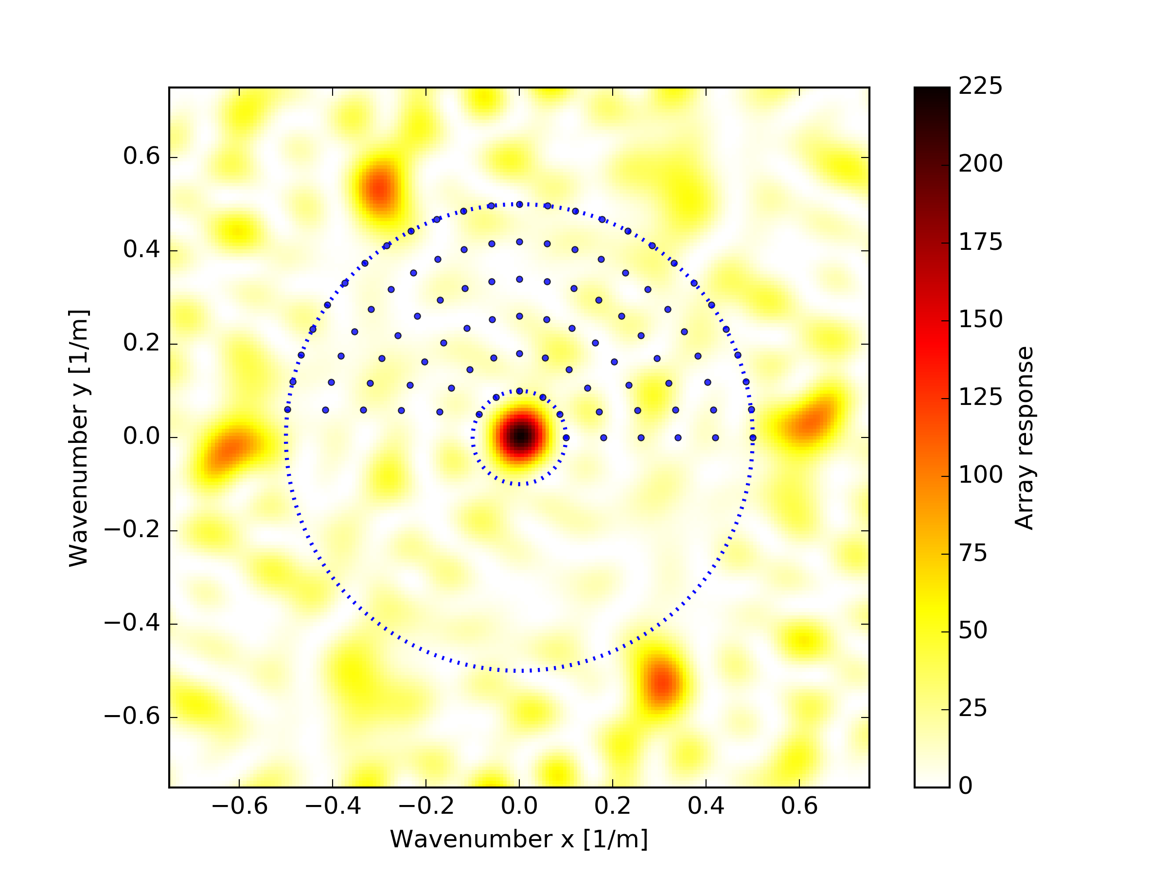
Array response.¶ |
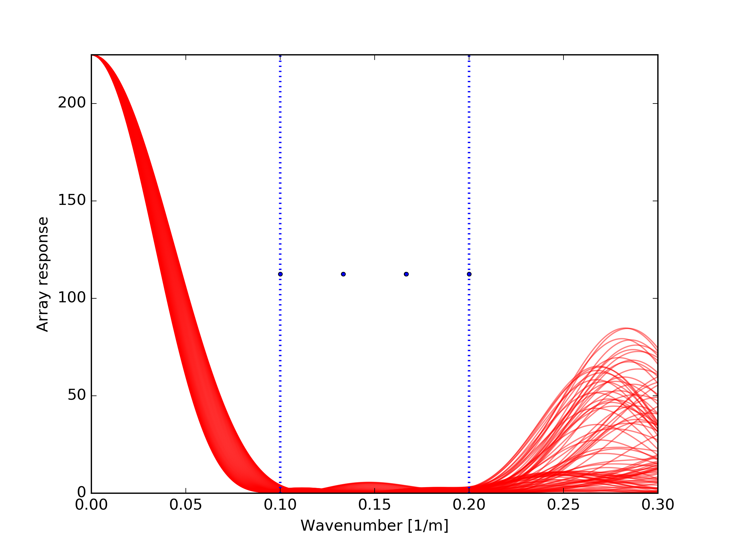
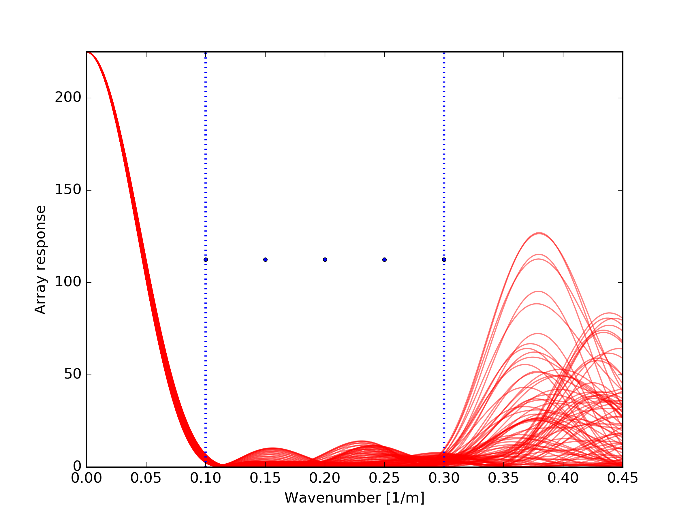
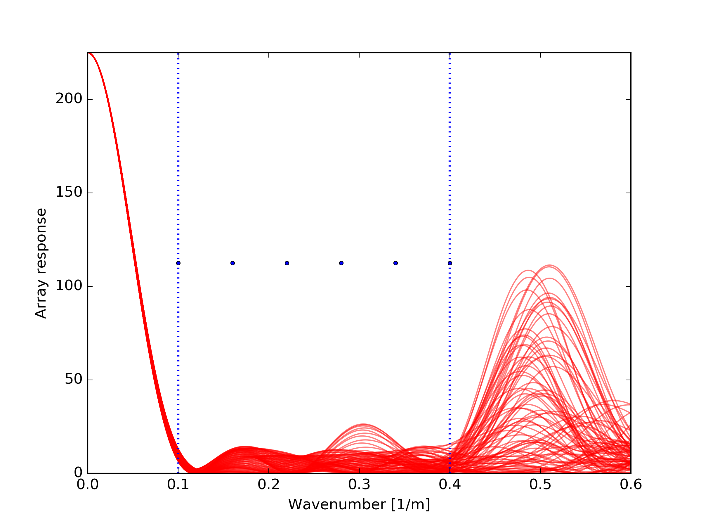
Array response, radial sections.¶ |
Kratio=3
Here we use  . This is an easy problem and a really good array is found.
Possible sensor positions and optimized array.¶ |
Array response.¶ |
Array response, radial sections.¶ |
Kratio=4
Here we use  .
.
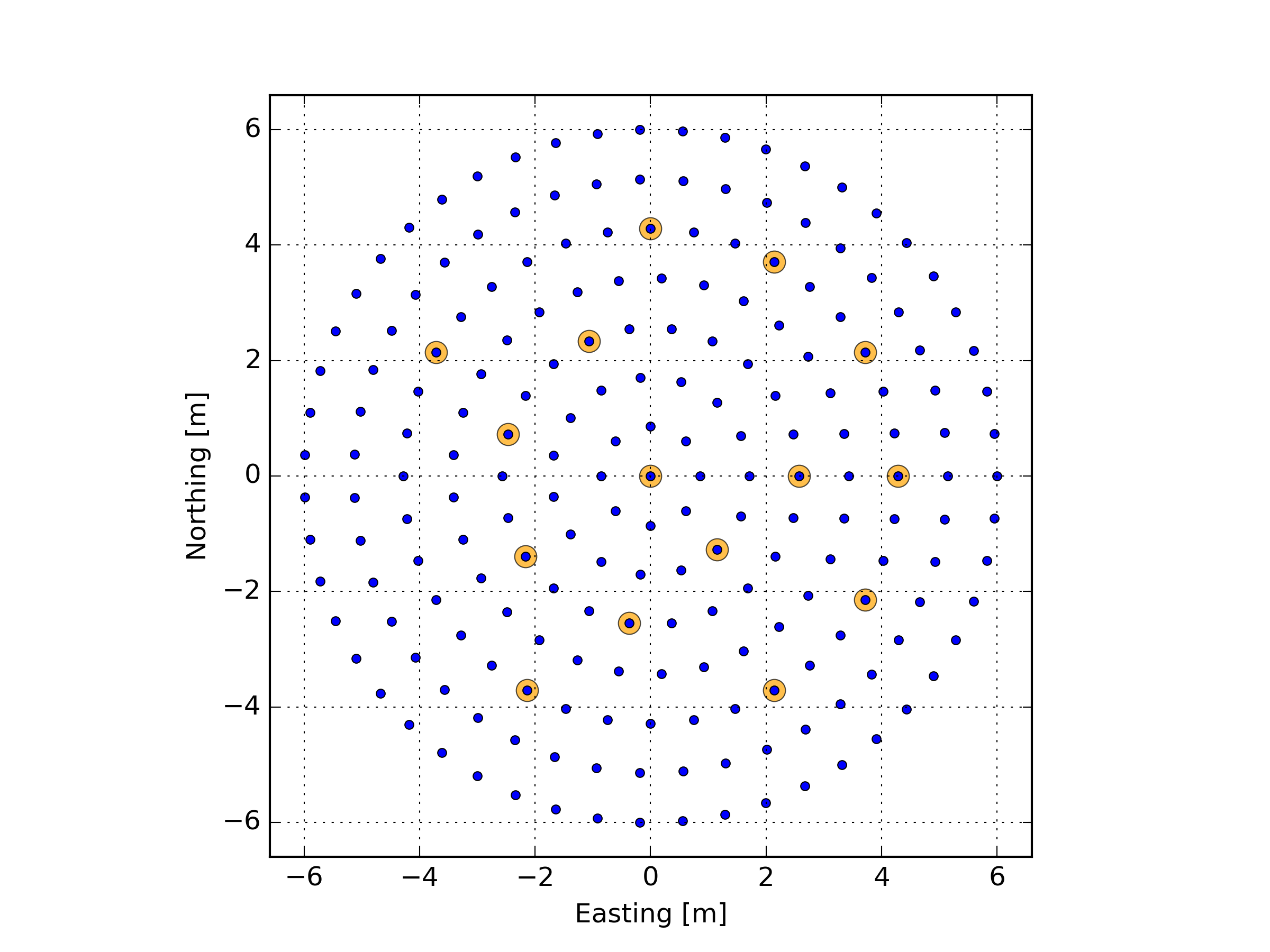
Possible sensor positions and optimized array.¶ |
Array response.¶ |
Array response, radial sections.¶ |
Kratio=5
Here we use  .
.
Possible sensor positions and optimized array.¶ |
Array response.¶ |
Array response, radial sections.¶ |
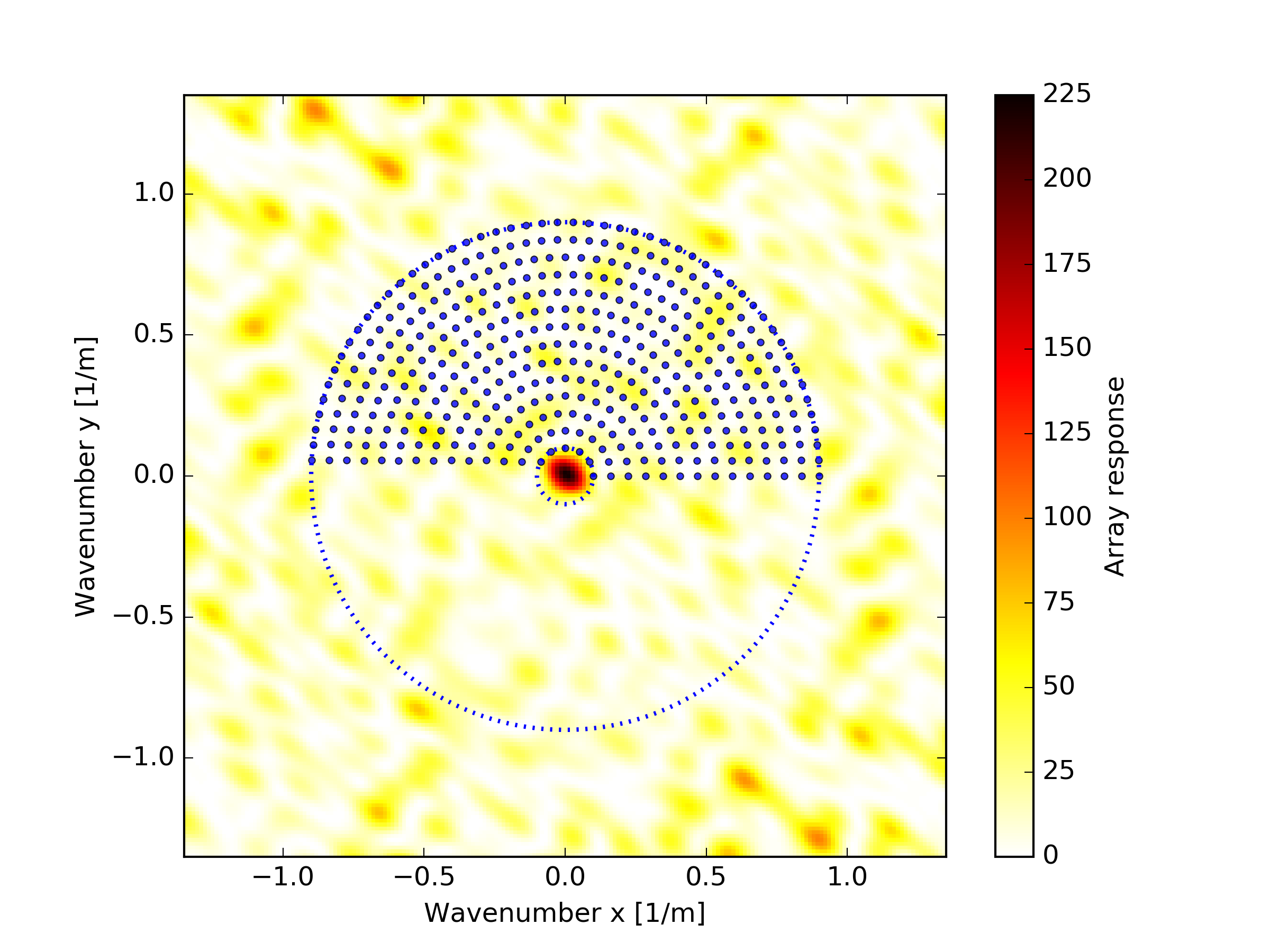
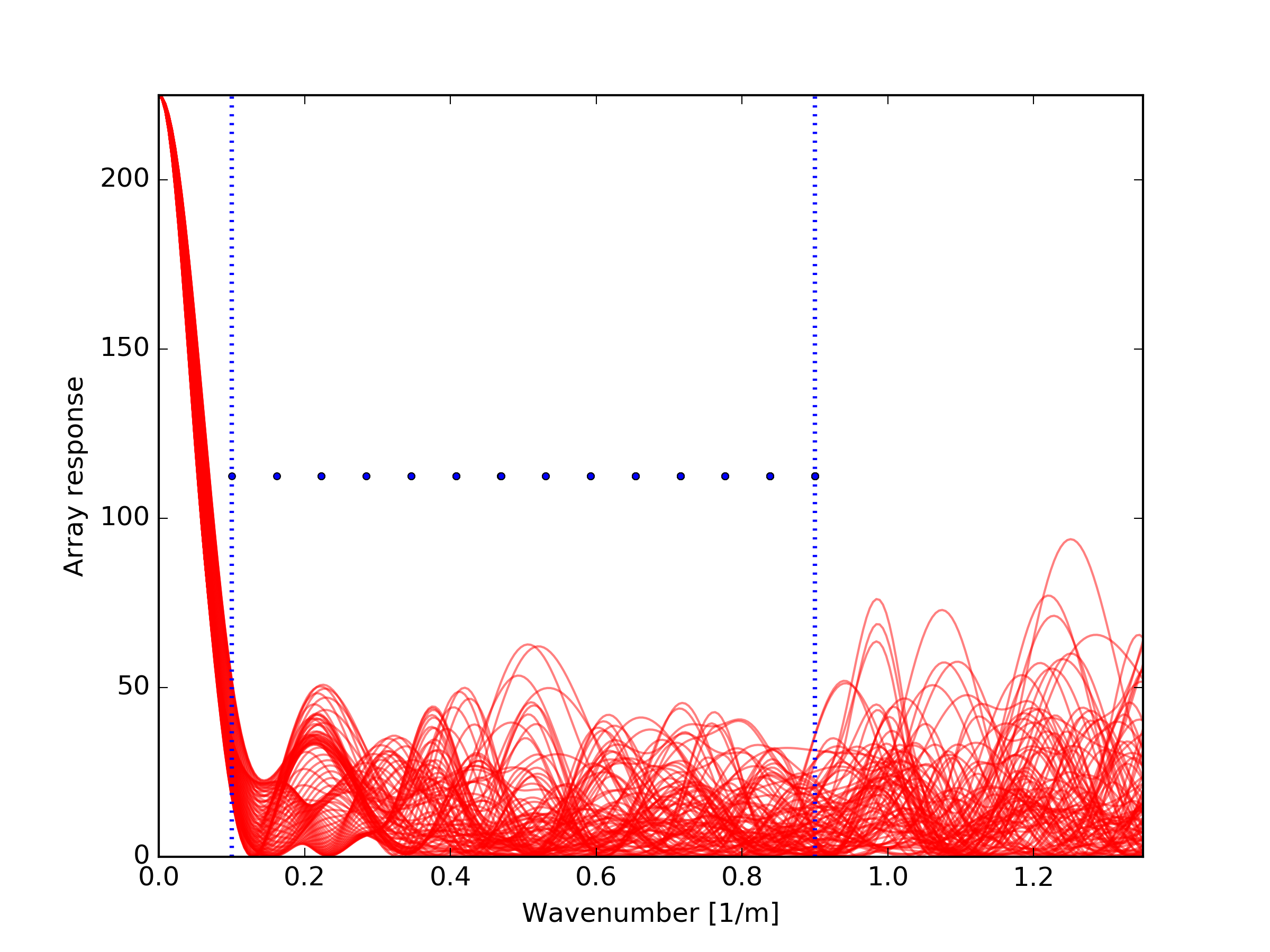
Kratio=9
Here we use  . The optimized array is not satisfactory as it exhibits large sidelobes in the minimization region.
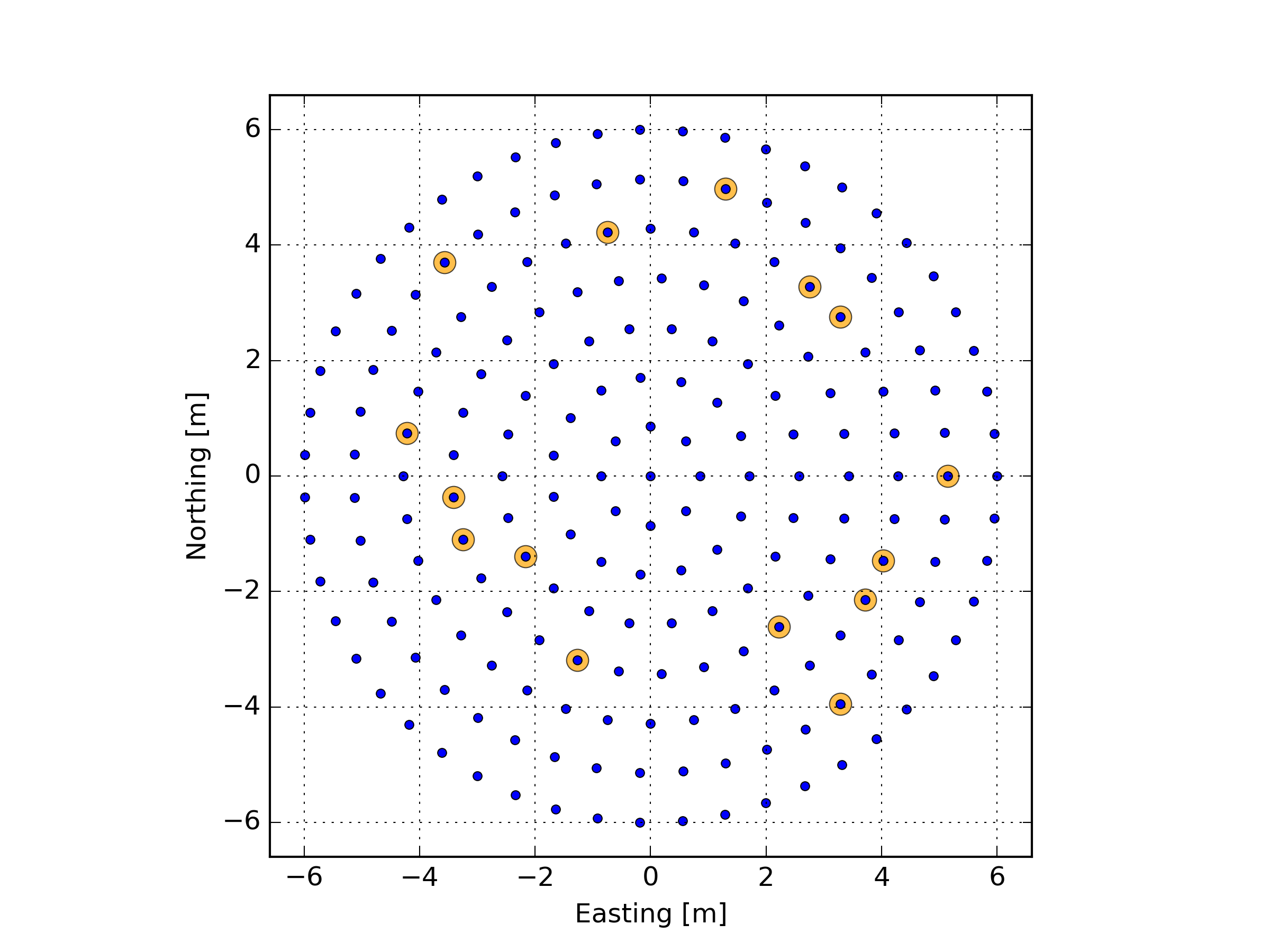
Possible sensor positions and optimized array.¶ |
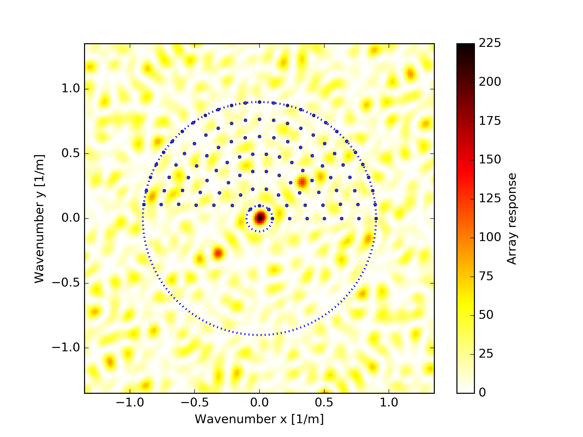
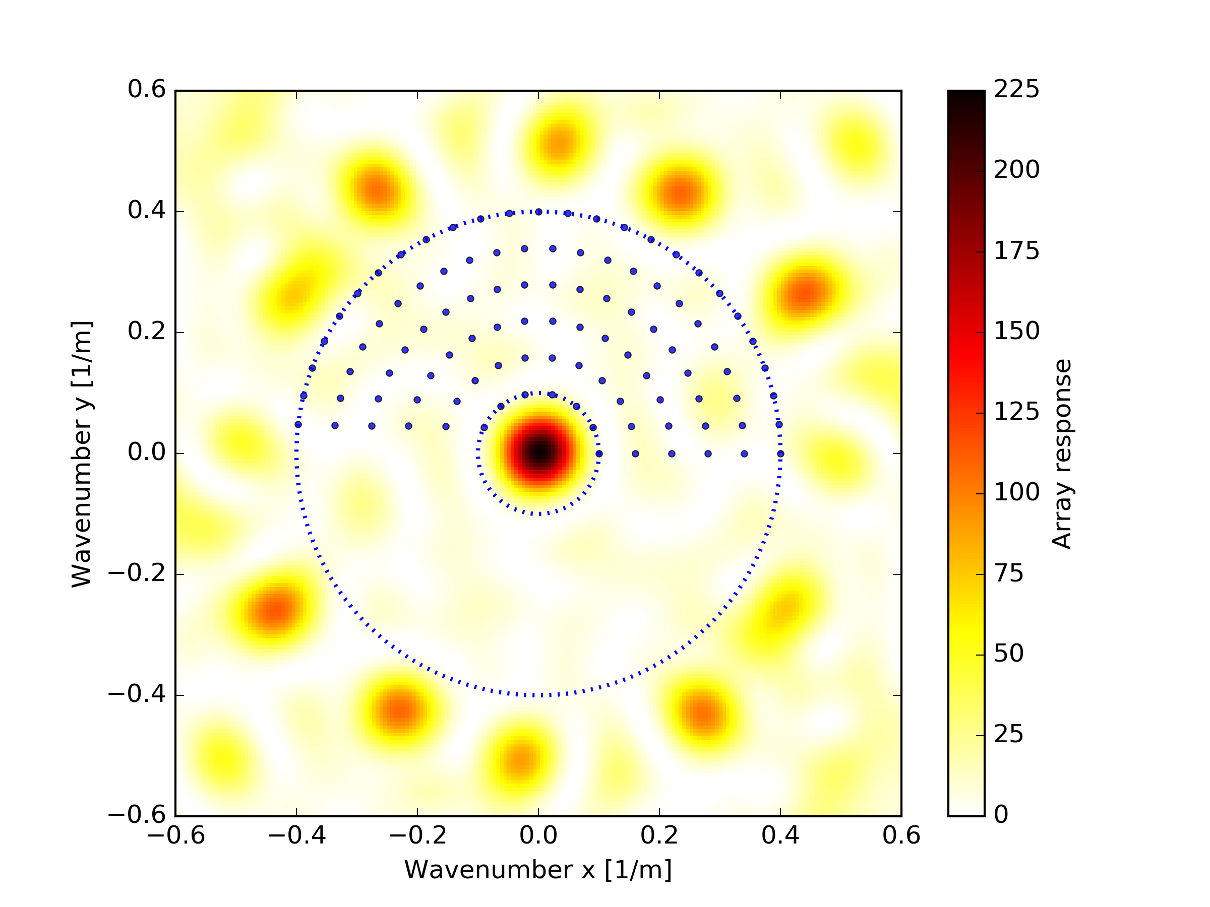
Array response.¶ |
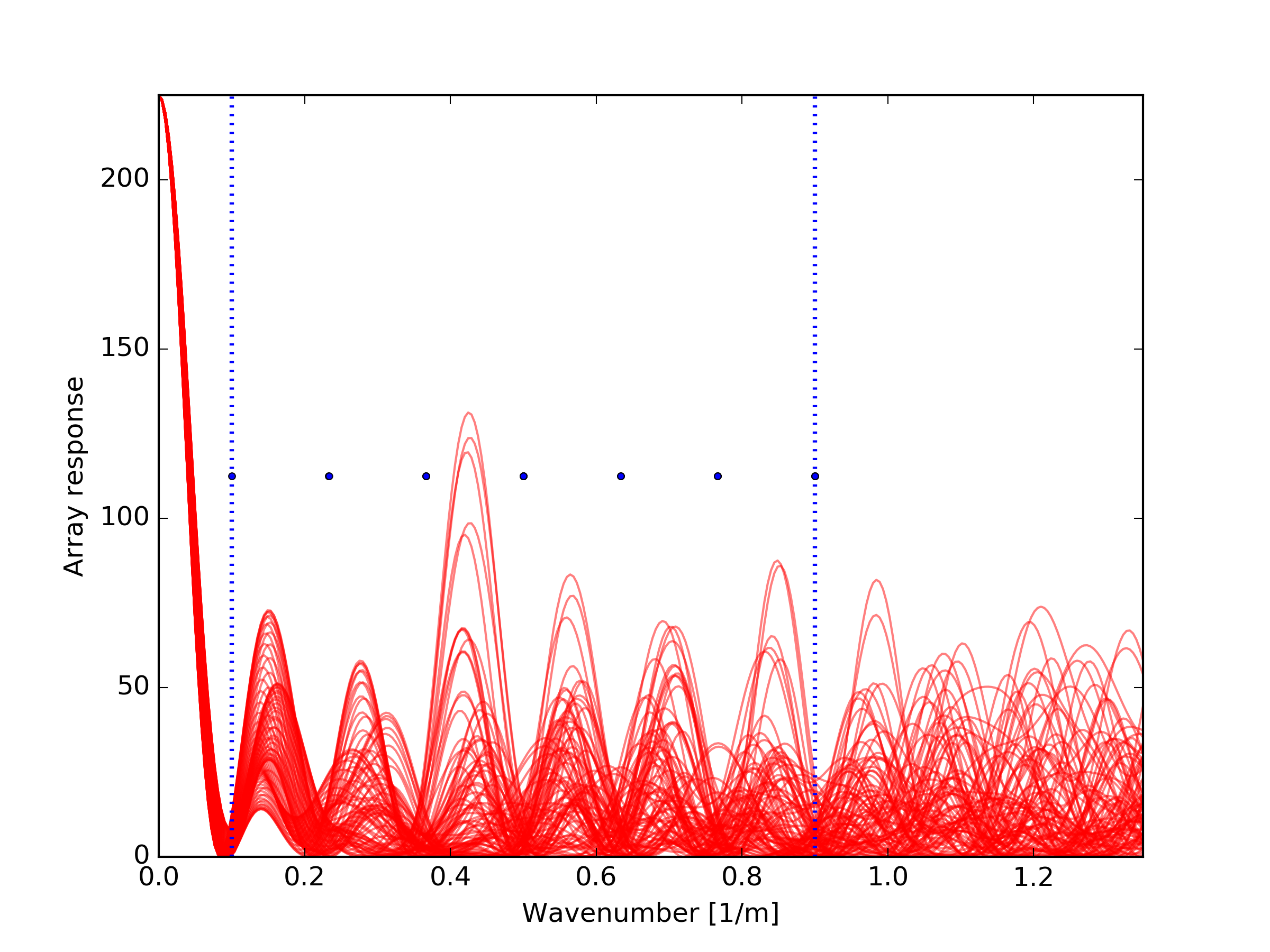
Array response, radial sections.¶ |
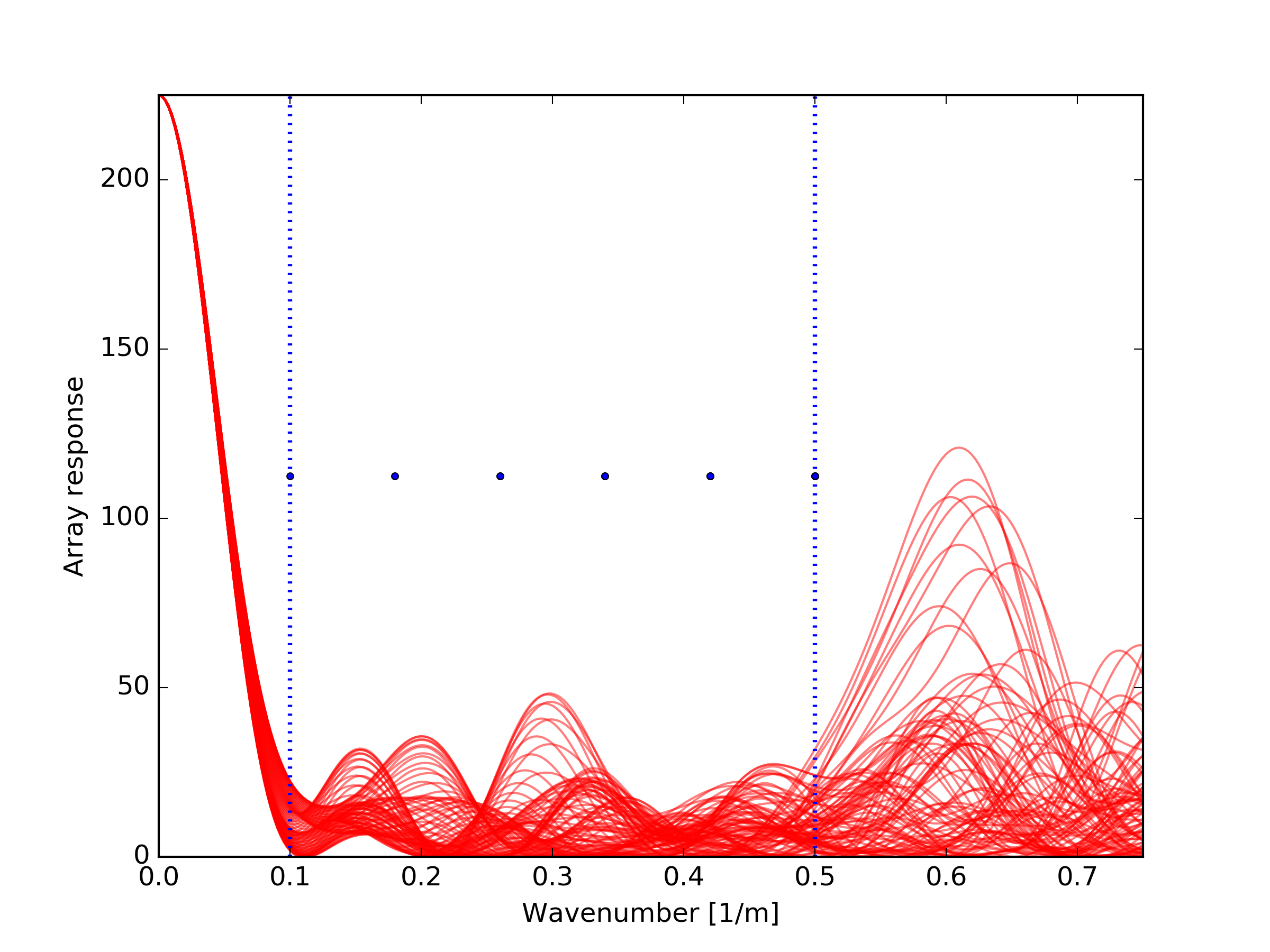
We observe that the sidelobes are especially large between the points of the frequency-domain grid. The algorithm is only sensitive to the value of the array response exactly at the points sampled (the blue dots shown in the array response plots).
To address this, we chose to increase the value of the parameter M, in order to obtain a finer frequency-domain grid. We set M: 400. Observe that there are  linear inequalities in Eq. (8). Increasing
 M will increase the computation and memory needed by the solver.
We also increase the time for the computation, setting TimeLimit: 3600. This may have only a marginal effect, sensor placement is a really hard problem and a small increase in computational power may have little effect. In any case, it will not harm.
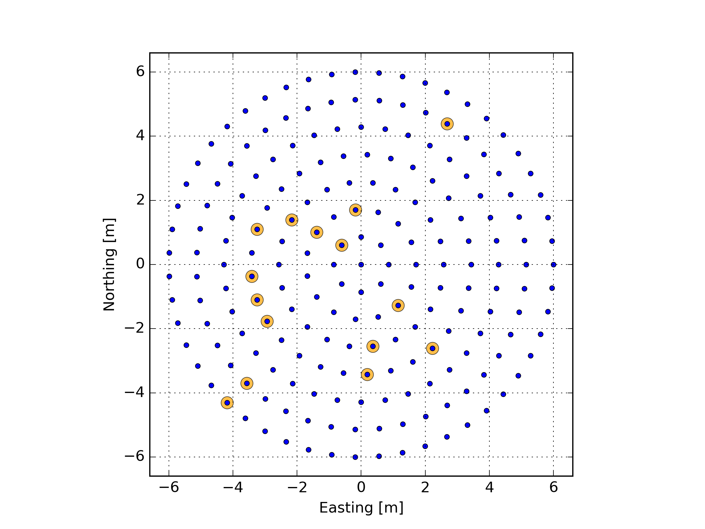
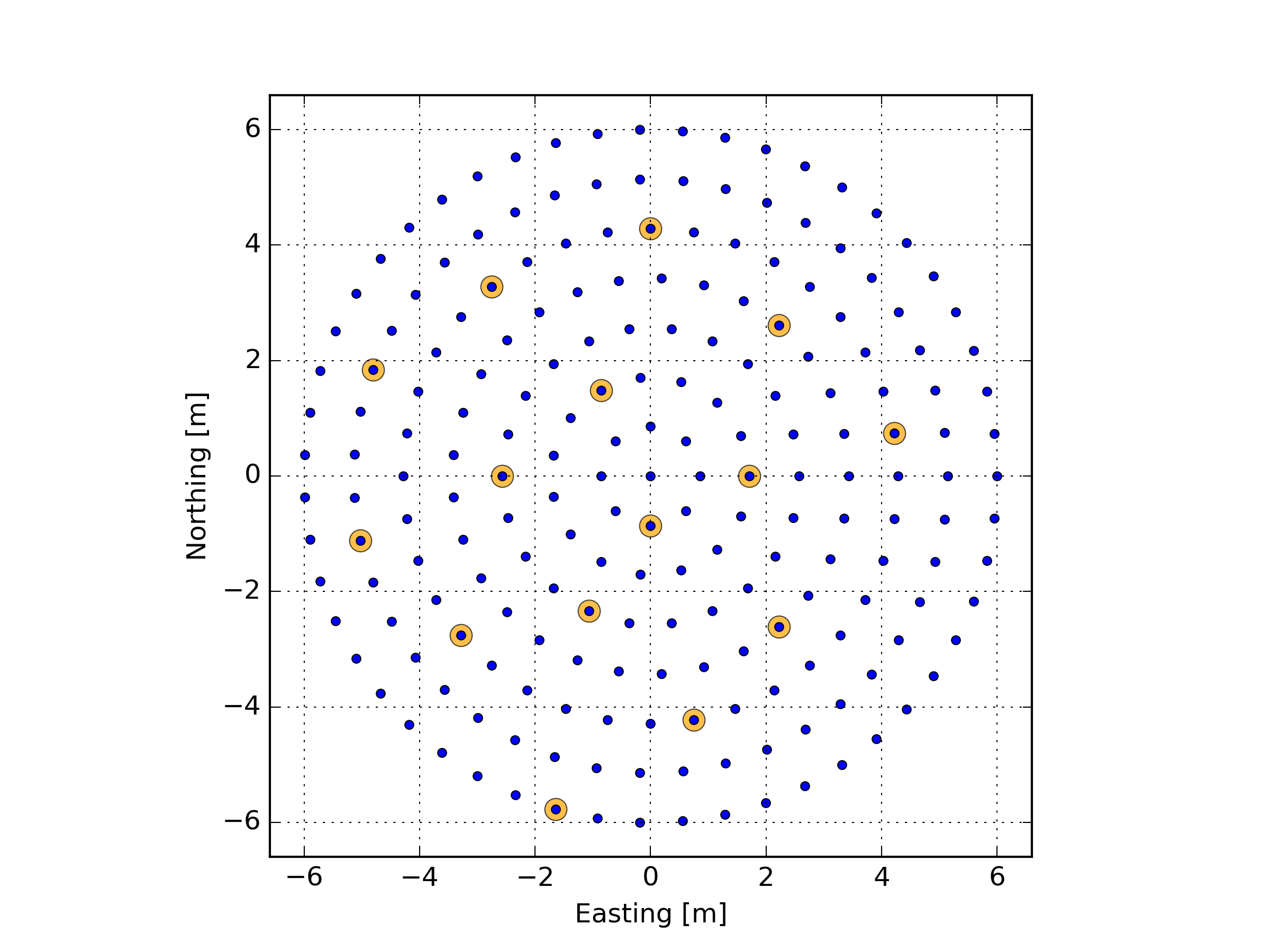
Possible sensor positions and optimized array.¶ |
Array response.¶ |
Array response, radial sections.¶ |
Possible positions from external file
In this example we load the possible sensor positions from an external file. This is extremely useful whenever there are physical obstructions in the area where we wish to deploy the array. Applications include surveying in urban areas.
grid from external file
too small aperture
too coarse M grid